The question:
Setting up a broadcasting antenna, how far does it reach? That’s the question we answer, without having to leave our cosy office. Even beyond that, we are simulating whole coverage networks:
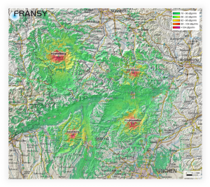
Field strength levels generated by 4 transmitters and simulated over location
That means in general, we calculate a prediction on how electromagnetic waves spread out. The underlying algorithm is called “the wave propagation model” which we constantly calibrate by different measurement campaigns.
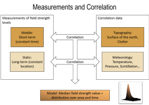
Two kinds of measurement data (on the left) are being correlated with available world data (on the right) to form a model that predicts a median field strength and distributions over location and time
To capture the variability of the field strength over location and time, two principal measurement data are needed:
- Long-term measurements over several years at a constant site
- Mobile measurements during a short time period at different locations
Static Long-term Measurements
We are interested, how the field strength varies over a typical (average) year, mainly for estimating the interfering potential of a signal. Therefore, long-term measurements over several years at a static location are needed.
On our rooftop we’ve installed 7 antennas which measure the field strength of 17 frequencies (UKW and DVB-T2) constantly every minute. Up to now, we’ve collected data of the last 4 years and as we analyse the distribution of the field strength levels for distant transmitters (~100 km), we recognize that it is not Gaussian. Indeed, higher field strength levels are more likely to occur than lower levels.
By correlating the field strength levels with atmospheric anomalies, we are optimizing our prediction model.
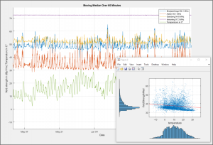
Example of field strength levels of 4 transmitters and temperature data over time (hourly moving median) with a correlation analysis of the whole year 2017.
Mobile Short-term Measurements
Besides the time variation of the field strength, the variation over location forms the obvious component of a field strength simulation. Looking at the first figure, the coverage map is made of tiny quadratic pixels and for each pixel a single field strength prediction has been calculated. A pixel in that figure corresponds to a square of 100 x 100 m and two results are needed: A median field strength and the location distribution inside the pixel.
Static Long-term Measurements
Modelling the field strength level in 2D
Dependency on location – correlation with topographic data
A so called 2D model only takes into account information along a direct line from receiver to transmitter as input parameters. The basic model for the calculation, which we use is the well-known Deygout-model1 extended by Meeks2 where, based on the topographic profile, the most important “knife edges” that damp the signal are calculated.
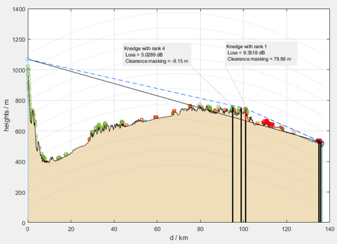
Modelling the median (50 % time) field strength based on a 2D height profile between transmitter and receiver by identifying most significant edges.
Dependency on time – correlation with atmospheric data
Sometimes, due to reflections in the atmosphere, the wave propagates further as usual which is called ducting effect. These high field strength levels are modelled by increasing a so-called k-factor which, multiplied with the earth radius, flattens the curvature to an effective earth radius reff:
reff = k * rearth
Afterwards, the same algorithm for identifying the edges is used as before.
This k-factor is strongly dependent on climate and surrounding. For example, in Germany around k = 1.3 are used for calculating the median field strength.
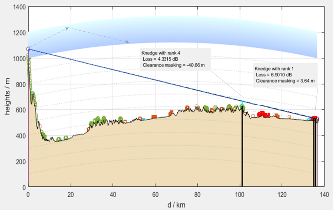
Modelling the field strength for k = 3 or << 1% of time. A duct (reflections are indicated in the blue ducting layer) is simulated by flattening the earth and using the same algorithm as before.
Reformulating the Question
Now we’ve seen that the field strength is highly varying, so the opening question has to be reformulated as follows:
Setting up a broadcasting antenna, how far does it reach for a certain percentage of locations in a pixel and a certain percentage of time during the year?
And broadcasters will answer pointing on the following picture: The green pixels show squares of 100 x 100 m wherein at 95 % of locations during 99 % of the year the signal is high enough.
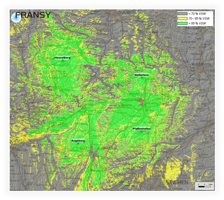
Coverage calculation: > 95 % means that in a green 100 x 100 m pixel over 95 % of locations are reaching the wanted level
But what is high enough? Even this question only can be answered statistically, but not now 🙂
- J. Deygout, „Multiple Knife-Edge Diffraction of Microwaves,“ IEEE Transactions on Antenna and Propagation, Bd. 14, Nr. 4, pp. 480-489, July 1966.
- M. L. Meeks, „VHF Propagation over Hilly, Forested Terrain,“ IEEE Transactions on Antennas and Propagation, Bd. 31, Nr. 3, pp. 483-489, 1983.